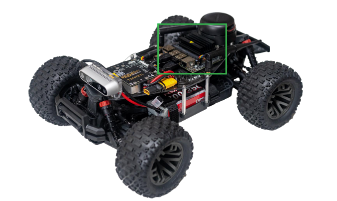
AEV Final Project
Given a an AEV equipped with Lidar, Jetson nano and an Intel Realsense camera, an algorithm for automous driving modes was made
General Description:
Part of the 3EY4 EE course at Mcmaster University, this final project course allowed me to develop many useful skills. This project requried:
- Setting up ROS
- Localization and Mapping with AEV
- Collision Avoidance and E-brake
- Wall Fallowing and Gap Methods of Autonomous Driving
- Virtual Barrier Autonomous Driving
- Computer Vision
Some of the most challenging parts of this project was understanding the kinematics and system dynamics of the vehicle and coordinate frames
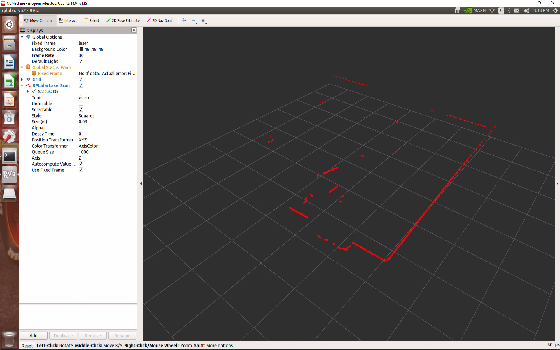
Lidar:
The following point cloud map of a hallway was created by visualising the measurements calculated by the onboard LIDAR sensor. In ROS, the lidar sensor has a node which publishes the data over a "/scan" topic, which the simulator and the visualiser are subscribed to.
Motor Controller:
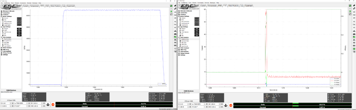
For this stage, the output for a certain input was studied. The motor controller could use either a speed command (top) or duty cycle command (bottom). The speed (left) and the voltage/current (right) output vary based on the type of input. As seen in the plots:
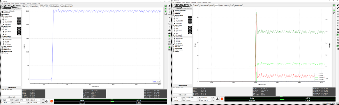
The speed command directly controls the speed of the motor with the use of an encoder while the duty cycle controls the PWM signal applied to the inverter. The duty cycle command settles quicker and has a lower RPM overshoot than the speed command, but requires a higher current overshoot
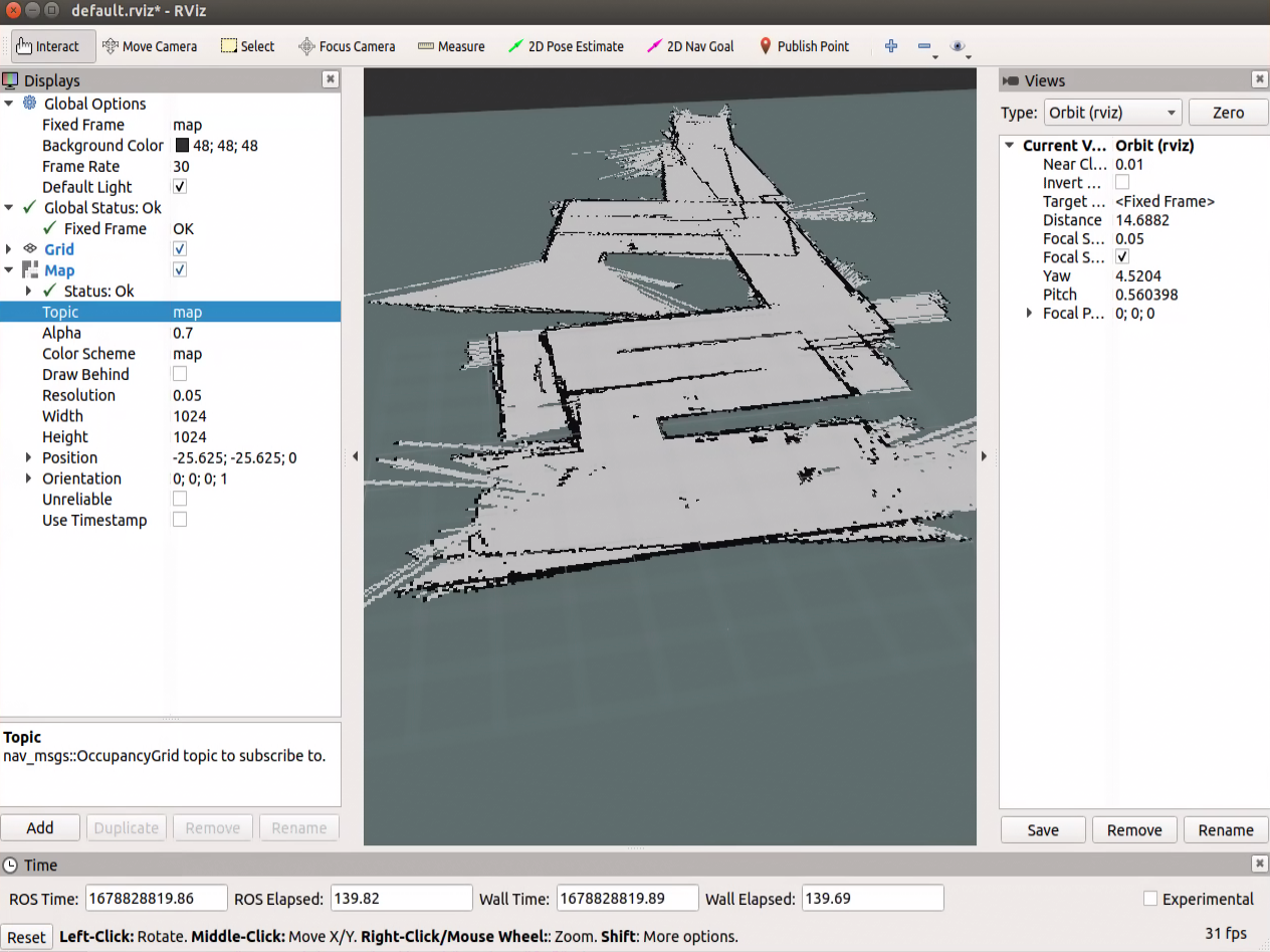
Mapping:
To the left, is an image of the map genereated by using the IMU data to calculate the wheel odomerty to track the position of the vehicle, and the LIDAR data is used to get the environmental details for said position using a Hector SLAM algorithm. The vehicle was manually driven using a joystick while Hector SLAM simultaneously used real-time LaserScan data to construct a map and localize the vehicle. The generated map displayed free spaces in grey and obstacles in black. Parameters such as map_update_distance_thresh and map_update_angle_thresh controlled how frequently the map was updated based on the vehicle’s movement. A key limitation of Hector SLAM was its lack of loop closure, meaning it could not recognize when the vehicle revisited previously mapped areas, leading to distortions and misalignments when returning to earlier parts of the environment.
Navigation (Wall Following):
A wall-following controller was implemented using LiDAR data to maintain a set distance from either the left wall, right wall, or a center offset between two walls. The controller dynamically adjusted the robot’s forward velocity based on the steering angle, allowing it to move faster on straight paths and slow down during turns. Three driving modes were available: Center Offset Mode, which balanced between two walls but introduced some zig-zagging; Left Wall Mode, which tracked the left wall and performed well in straight hallways but struggled around corners; and Right Wall Mode, which had similar characteristics. Tuning the controller's proportional (kp) and derivative (kd) gains significantly influenced the transient response, affecting overshoot, damping, and settling time. Ultimately, the center-offset method was selected as the best trade-off for handling turns despite minor steering oscillations. Additionally, a collision avoidance node was developed to enhance joystick-based manual control by automatically steering the robot away from obstacles detected using LiDAR scans. This node read parameters such as joystick axes, collision thresholds, LiDAR range, and control gains from a params.yaml file, subscribed to LiDAR, odometry, and joystick messages, and published safe Ackermann steering and speed commands. By preprocessing LiDAR data to focus on the front 180° field of view and detecting obstacles within a critical distance (d_obs), the node calculated repulsive forces using a potential field method. It then blended these corrections with joystick inputs, ensuring that users could manually control the robot while maintaining collision-free navigation.
Navigation (Autonomus Driving):
The autonomous algorithm developed in this project aims to improve wall-following behavior and optimize obstacle avoidance in a robot using LIDAR data and control strategies. The algorithm primarily focuses on selecting an optimal heading direction and adjusting the robot's steering and velocity based on its environment.
Initialization and Preprocessing: The algorithm starts by loading the necessary files and parameters, including LIDAR configurations. In particular, the GapBarrier class is used to identify and process LIDAR points within a 180° field of view (FOV). The preprocess_lidar function processes these points, adjusting them based on a defined safe distance to avoid obstacles.
Gap Detection and Optimization: The next step is to identify gaps in the data, which represent potential paths. The find_max_gap function identifies the largest gap, and the find_best_point function computes the optimal direction to move. Rather than choosing the furthest point in the largest gap, the algorithm uses a weighted average of points within the gap to minimize erratic behavior caused by noisy or non-uniform LIDAR data.
Quadratic Optimization: The optimization for virtual barriers is achieved through a quadratic programming formulation. The getWalls function uses the quadprog solver to compute the virtual walls that the robot should maintain for safe navigation. The algorithm takes into account control parameters like proportional and derivative gains (k_p, k_d) to adjust the transient behavior of the system, ensuring smoother and more stable responses during wall-following.
Control System and Dynamic Adjustment: The system adjusts the robot's velocity dynamically based on its steering angle. It has three driving modes: center offset (balanced between two walls), left wall mode, and right wall mode. The center offset mode is selected as the best trade-off, as it handles turns better despite some oscillation. Control parameters like velocity_high, velocity_medium, and velocity_low adjust speed based on the steering angle.
Obstacle Avoidance and Wall Markers: Collision avoidance is incorporated by integrating a repulsive force model that steers the robot away from obstacles detected by LIDAR. The system also uses rviz to visualize the robot's virtual walls and travel direction, helping to represent the environment for simulation.
Fine-Tuning and Improvements: The vehicle's response to parameters like k_p, k_d, n_pts_l, n_pts_r, and safe_distance was observed and adjusted during experiments. For instance, k_p and k_d affect the system's speed and stability, while n_pts_l and n_pts_r define how precise the robot’s trajectory is. Modifying the safe_distance parameter made the robot more selective in choosing gaps, enhancing its accuracy in avoiding obstacles.
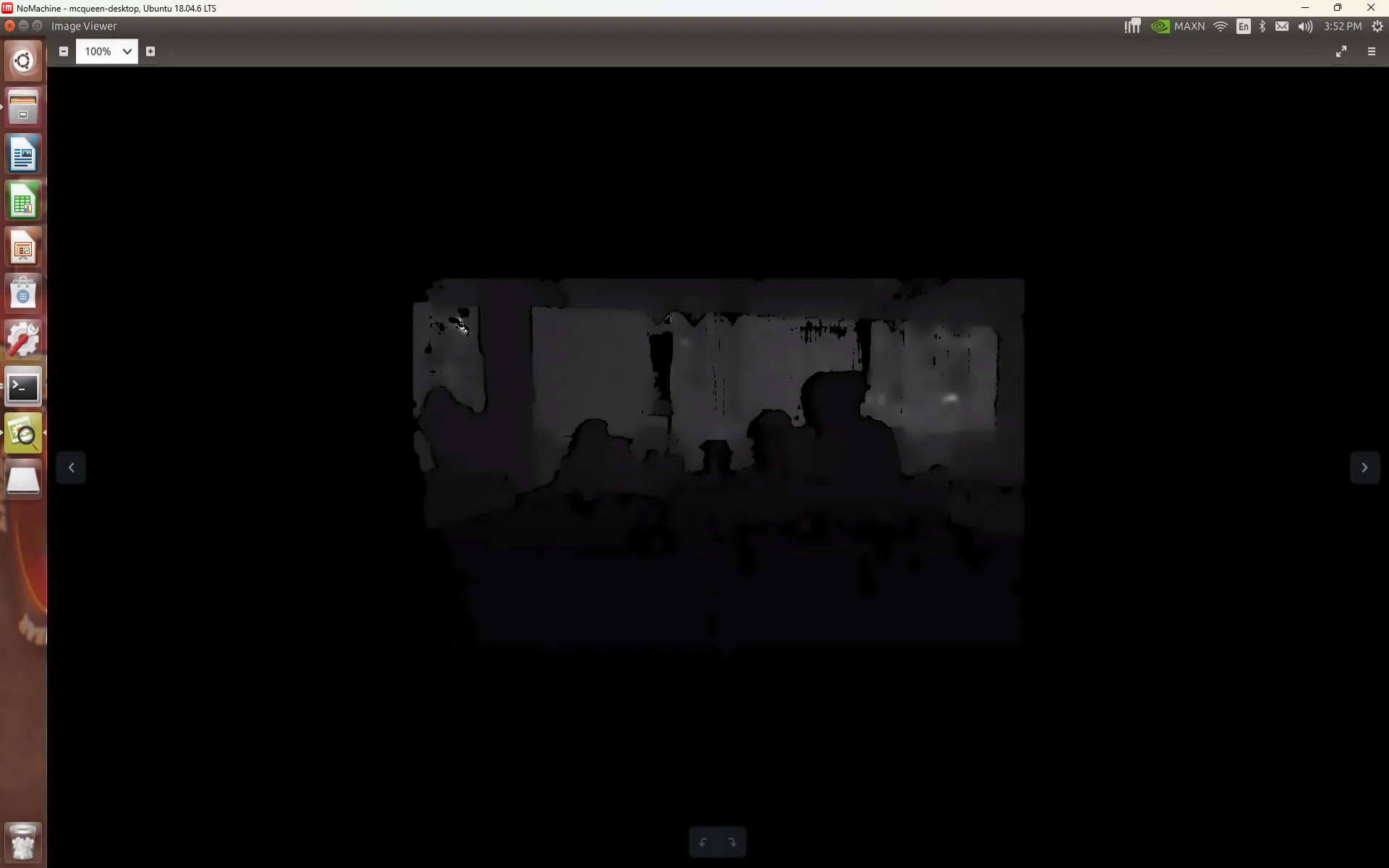
Implementing the Camera:
Up until now, in the labs we have been performing autonomous functions using only the lidar sensor as the cars input, this allowed us to implement methods to drive autonomously with wall following or finding the desired heading direction based on the open space detected by the lidar sensor. Although these are functional, they are still limited in many ways, for example when using the desired heading direction, the car will not see a wall that is past a large open gap and run into it. This can be solved by implementing the intel real sense depth camera. Using the depth camera, we can tell the AEV if an object is present with the distance measurement measured by the camera. Implementing this with the lidar sensor will improve the reliability of autonomous mode
A Node was created to subscribe to the camera topic image_rect_raw, and a new function called “preprocess_camera” was developed to replace the previous “preprocess_lidar” function. Additionally, the “lidar_callback” function was renamed to “camera_callback.” Within the new “preprocess_camera” function, the bottom half of the camera image was extracted and processed, with the possibility of neglecting certain pixels that detect the ground, depending on the results of testing. For each column of the camera image, the pixel with the smallest depth was saved into a new array. Using this array, each pixel was converted into an equivalent distance and angle measurement, with the angle calculated based on the known focal length of the camera and the pixel size.
The node functions as intended; it provides collision assistance similar to when using the lidar scans. The depth camera collision assistance was able to track more objects but was must less responsive. This can be attributed to the image processing component of the code, which is very heavy load in terms of calculations.